Measures of Central Tendency and Dispersion

Overview

Definition

Measures of central tendency are single values that attempt to describe a data set by identifying the central or “typical” value for that data set.

• Colloquially described as “averages”
• Most common measures:
  • Mean
  • Median
  • Mode

Data distribution and measures of dispersion

• In any data set, the data are distributed over a certain range.
• Based on this distribution, one can determine how close most of the data are to the mean or how spread out the data are; this dispersion can be measured in several ways, including:
  • Percentiles
  • Standard deviations
• Typically, certain data points are more common in the data set (those close to the average), while others are rare (i.e., outliers).
• How these data points distribute can be classified as:
  • Normal
  • Nonnormal
• Normal distributions have certain characteristics that can help clinicians determine how “abnormal” a particular finding is: For example, is a particular lab result within the range of “normal” or does the finding suggest a disease state?

Mean, Median, and Mode

Mean

Definition:

Mean is the sum of all measurements in a data set divided by the number of measurements in that data set.

• The arithmetic average of all observed values
• Can be incorporated in more complex statistical analyses
• The most affected by outliers
• The mean of a random sample is an unbiased estimator of the population from which it came.
• The mean is the mathematical expectation and may not even be present in a sample (as opposed to the mode or median).

Equation:

$$ Mean = \frac{Sum\ of\ all\ values\ in\ the\ data\ set}{Total\ number\ of\ values\ in\ data\ set} $$ $$ Mean = \frac{x_{1}+x_{2}+x_{3}+…+x_{n}}{n} $$

Example:

Find the mean of the following data set: 1, 1, 1, 3, 5, 5, 7, 19.

Answer: There are 8 numbers in this data set. To calculate the mean, add up all the numbers and divide by 8:

$$ Mean = \frac{1+1+1+3+5+5+7+19}{8}=\frac{42}{8}=5.25 $$

Median

Definition:

After arranging the data from lowest to highest, the median is the middle value, separating the lower half from the upper half of the data set. 

• Serves as the central dividing point of the data
• Does not lend itself to more complex statistical inference
• If the number of values in the sample is even, then the median is the average of the 2 numbers in the middle.
• More affected by outliers than the mode but less so than the mean
• The median and the mode are the only measures of central tendency that can be used for ordinal data.

Equation:

To find the median, arrange the values from lowest to highest, then use the following equation to determine which “position” in order represents the median:

$$ Median = \left \{ \frac{(n+1)}{2} \right \} $$

where n = the number of values in the data set. 

Example:

Find the median of the following data set: 1, 5, 1, 19, 3, 1, 7, 5.

Answer: There are 8 numbers in this data set. To find the median, first arrange the numbers in order: 1, 1, 1, 3, 5, 5, 7, 19.  Next, determine which “position” represents the median. To do this, use the formula (n + 1) / 2. There are 8 numbers in this data set, so n = 8. Therefore, the median will be: (8 + 1) / 2 = 4.5. The median is between the 4th and 5th numbers, which are 3 and 5 (visually: 1, 1, 1, 3, 5, 5, 7, 19). So the median in this data set is 4.

Mode

Definition:

 The mode is the value that occurs most frequently in the data set.

• To find the mode, set up a frequency table to determine which value occurs most often in the data set (see example below).
• More useful for qualitative analysis (nonnumerical) than for statistical analysis
• A distribution may have a mode at > 1 value.
• The only central tendency that can be used with nominal data
• Least affected by outliers
• Cannot be obtained by mathematical equations

Example:

Find the mode of the following data set: 1, 5, 1, 19, 3, 1, 7, 5.

Answer: Identify the number that appears most often. This can be done by setting up a frequency table:

Table: Frequency table

Data point	Frequency (how often the data point occurs in the sample)
1	3
3	1
5	2
7	1
19	1

Mnemonic:

MOde is the value that is in the set MOst often.

Summary

Table: Summary of the mean, median, and mode

Type	Description	Example	Result
Mean	Total sum of numbers divided by number of values	(8 + 4 + 10 + 4 + 4 + 5 + 4 + 5 + 6) / 9	5.5
Median	Middle value that separates higher half from lower half	4, 4, 4, 4, 5, 5, 6, 8, 10	5
Mode	Most frequent number	4, 4, 4, 4, 5, 5, 6, 8, 10	4

Measures of Dispersion: Percentiles and Standard Deviations

Dispersion is the size of distribution of values in a data set. Several measures of dispersion include a range, quantiles (e.g., quartiles or percentiles), and standard deviations.

Based on quantiles

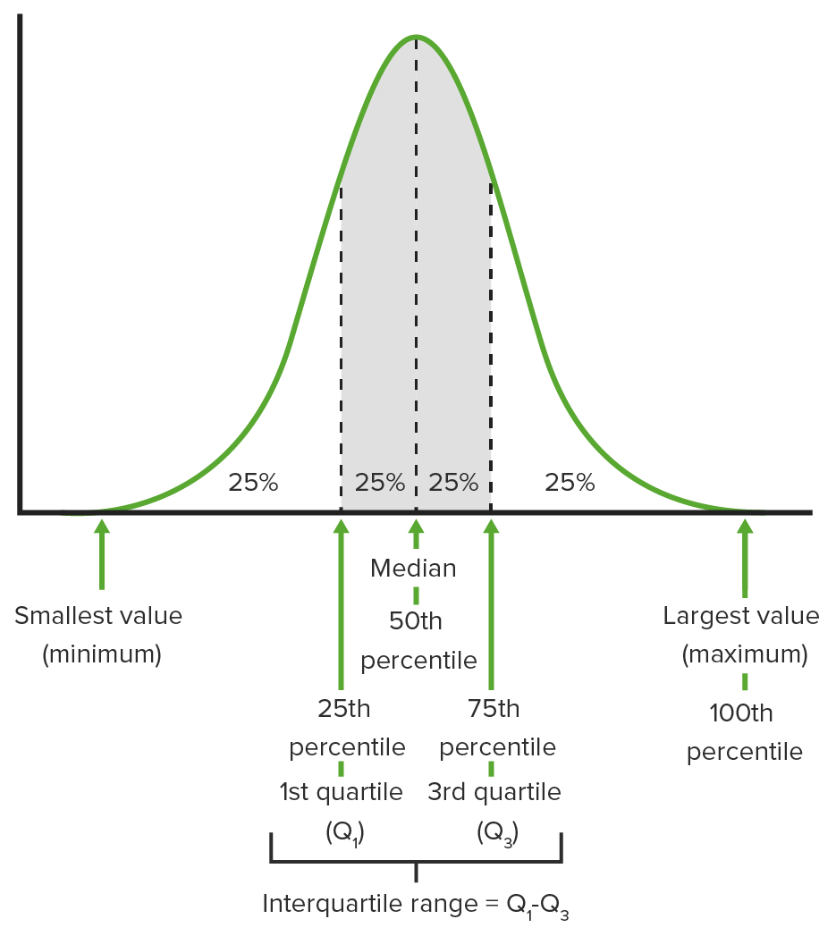
• A quantile divides a data set into equal proportions and represents the proportion of data at or below that point; special quantiles are:
  • Quartiles: The data set is divided into 4 quarters.
  • Quintiles: The data set is divided into 5 sections.
  • Percentiles: The data set is divided into 100 sections.
• For example:
  • The 50th percentile is the median.
  • The 75th percentile is the point below which 75% of the values in your data set are found.
  • The 25th percentile is the point below which 25% of the values in your data set are found.
• The set of data between the 25th and 75th percentiles (the 1st and 3rd quartiles) is known as the interquartile range.
• Quantiles can be applied to any continuous data set.
• Uses include:
  • Clinical: growth curves Growth Curves Short Stature in Children
  • Research Research Critical and exhaustive investigation or experimentation, having for its aim the discovery of new facts and their correct interpretation, the revision of accepted conclusions, theories, or laws in the light of newly discovered facts, or the practical application of such new or revised conclusions, theories, or laws. Conflict of Interest: box plots Box plots Shows the spread and centers of the data set. Statistical Tests and Data Representation (graphical displays of data demonstrating the range of numerical results observed in a study)

Based on the mean: standard deviations

Definition: The standard deviation (SD) is a measure of how far each observed value is from the mean in a data set.

• The standard deviation is typically abbreviated as SD, or it may be represented by the lower case Greek letter sigma (σ).
• Can be used when the distribution of data is approximately normal, representing a bell curve
• A low SD means that the data are closely clustered around the mean.
• A high SD means that the data are spread out over a wider range of values.
• Used to determine whether a particular data point is “standard/expected” or “unusual/unexpected”:
  • The more SDs a data point is from the mean, the more “unusual” that data point is.
  • Can help distinguish whether a result is within the “expected variation” or is more of an outlier
• Standard deviaitions can be appreciated visually as the area under the curve (AUC):
  • 1σ = approximately 34% of the AUC = approximately 68% of results are within 1 SD of the mean
  • 2σ = approximately 48% of the AUC = approximately 95% of results are within 2 SD of the mean
  • 3σ = approximately 49.8% of the AUC = approximately 99.7% of results are within 3 SD of the mean

Equation:

Mathematically, the SD can be calculated using the following equation:

$$ \sigma = \sqrt{\frac{\sum (\chi _{i}-\mu )^{2}}{N}} $$

σ = population standard deviation
Ν = the size of the population
χᵢ = each value from the population
μ = the population mean

Calculations (using the equation):

1. Find how far each value is from the mean, then square this value. (Note: This is the square of the variance.)
2. Find the sum of these squared values.
3. Divide this sum by the total number of values in the data set.
4. Take the square root of that number to find the SD.

Data Distribution

Data distribution describes how your data cluster (or don’t cluster). Data tend to cluster in certain patterns, known as distribution patterns. There is a “normal” distribution pattern, and there are multiple nonnormal patterns. Different statistical tests are used for different distribution patterns.

Data distribution

Normal distributions differ according to their mean and variance, but share the following characteristics:

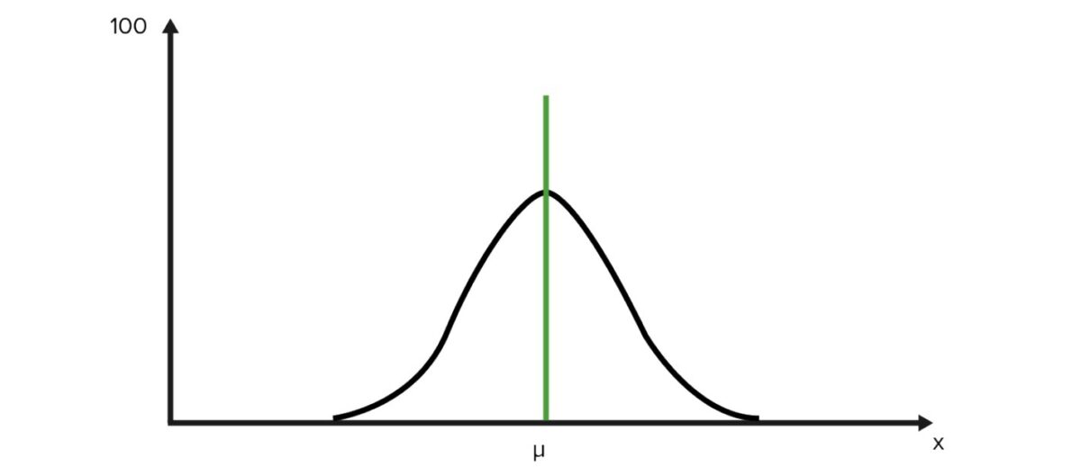
• Classic symmetrical Symmetrical Dermatologic Examination “bell curve” shape: 
  • All measures of central tendency are equal (mean = median = mode).
  • 50% of values are less than the mean; 50% of values are greater than the mean.
• Follows the central limit Limit A value (e.g., pressure or time) that should not be exceeded and which is specified by the operator to protect the lung Invasive Mechanical Ventilation theorem, which works as follows:
  • Take a sample from the population and calculate the mean; then put that sample back into the population, take a new sample and calculate the mean; do this over and over again.
  • Some means will be very common, representing the true mean of the population. Other means will be very uncommon; these are farther from the true mean of the population.
  • If you graph the frequency of each mean you obtain, you will generate the classic bell curve shape.
• All normal distributions have the same shape because they have the same data distribution:
  • About 68% of values are within 1 SD of the mean.
  • 95% of the data fall within 2 SD of the mean.
  • 99.7% of the data fall within 3 SD of the mean.
• The area under the curve represents the probability Probability Probability is a mathematical tool used to study randomness and provide predictions about the likelihood of something happening. There are several basic rules of probability that can be used to help determine the probability of multiple events happening together, separately, or sequentially. Basics of Probability of obtaining a certain value, so the total area under the curve = 1.
• Things that tend to follow normal distributions:
  • People’s heights, weights, and BPs
  • Results on exams
  • Sizes of objects produced by machines

Nonnormal distribution

Many processes follow a nonnormal distribution, which can be due to the natural variations or errors in the data.

Common distributions:

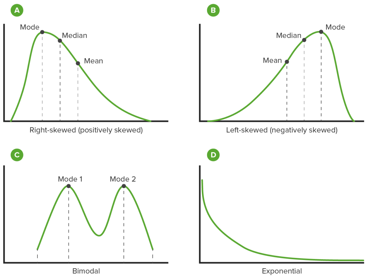
• Skewed:
  • Right-skewed (or positively skewed): 
    • Tail spreads out to the right.
    • Mean > median > mode
  • Left-skewed (or negatively skewed):
    • Tail spreads out to the left.
    • Mode > median > mean
  • Note: Tails may act as outliers and adversely affect the statistical tests.
• Bimodal: 
  • A distribution with 2 “peaks” (representing the 2 modes in the data)
  • Suggests 2 different populations
• Exponential:
  • There are few very large values and many more small values.
  • Often deals with the amount of time until a specific event occurs, for example:
    • How many months a car battery lasts until it dies
    • Radioactive decay

Reasons why data may have a nonnormal distribution:

• Many data sets naturally fit a nonnormal model (e.g., bacteria Bacteria Bacteria are prokaryotic single-celled microorganisms that are metabolically active and divide by binary fission. Some of these organisms play a significant role in the pathogenesis of diseases. Bacteriology growth follows an exponential distribution)
• Data collection methods or other methods may be at fault.
• Outliers can cause data to become skewed.
• Multiple distributions may be combined, giving the appearance of a bimodal or multimodal distribution.
• Insufficient data can cause a scattered distribution.

References

1. Katz, D., et al. (2014). Describing variation in data. In Katz, D. et al. (Eds.), Jekel’s Epidemiology, Biostatistics, Preventive Medicine, and Public Health. Elsevier. Pp. 105–118.
2. Weisberg H. F. (1992) Central tendency and variability. Sage University Paper Series on Quantitative Applications in the Social Sciences. SAGE Publications, Inc; 1st ed., p. 2.
3. Johnson N. L., Rogers, C. A. (1951). The moment problem for unimodal distributions. Annals of Mathematical Statistics 22:433–439.
Create your free account or log in to continue reading!
Sign up now and get free access to Lecturio with concept pages, medical videos, and questions for your medical education.
User Reviews
Unwrap New Skills This Holiday 🎄 Save 30% on all plans now!